How Data Science Measures Market Shocks: The Israel Airstrikes Case Study
A step-by-step event study measuring how the June 2025 Israeli and U.S. strikes on Iranian targets moved Israel's equity market.
Data science provides a powerful lens for understanding real-world events—like Israel's strikes on Iranian nuclear and military sites that began on 13 June 2025—but how did these events impact Israel's financial markets?
In this case study, we examine how the Tel Aviv Stock Exchange, as proxied by the iShares MSCI Israel ETF (EIS), responded to the escalation. Using a classic event-study framework, we quantify the impact of these airstrikes on Israeli market returns—leveraging nothing more than public data and Python.
But this isn't just about geopolitics. The same techniques apply across industries:
- When Uber rolls into a new city, how do local taxi markets respond?
- After a corporate fraud revelation, does investor confidence bounce back—or crater?
- How does a staggered policy rollout across regions shape consumer behavior?
Whether it's war, innovation, or scandal, event studies allow us to ask: What changed—and was it because of this?
Key finding (preview): The Israeli market dipped slightly on the strike day but rebounded sharply the very next session—showing resilience, not panic.
This analysis draws on foundational tools from applied econometrics and finance, including:
- 🗓️ Event-day indicators to isolate the effect of the June 13 strike
- 📈 Time-series regression to estimate abnormal returns
- 🎯 Placebo inference to test if the observed movement was statistically significant
Data Collection & Preparation
To measure the market impact, we'll start by pulling daily returns data from Yahoo Finance using three ETFs:
- EIS – iShares MSCI Israel ETF (target asset)
- VOO – Vanguard S&P 500 ETF (U.S. benchmark)
- VXUS – Vanguard Total International Stock ETF (global benchmark)
We include VOO and VXUS to control for broad U.S. and ex-U.S. market movements, helping us isolate the strike's specific effect on Israeli equities.
import yfinance as yf
import pandas as pd
import statsmodels.api as sm
import numpy as np
import matplotlib.pyplot as plt

# Define tickers and time range
tickers = ["EIS", "VXUS", "VOO"]
start = "2023-01-01"
end = "2025-06-22"

# Download adjusted closing prices
df = yf.download(tickers, start=start, end=end, auto_adjust=True)["Close"]
Next, we compute daily returns to feed into our regression model:
# Calculate daily returns
returns = df.pct_change().dropna()
Our event date is 13 June 2025—the day Israel launched airstrikes on Iranian targets:
# Define the event date
event_date = pd.to_datetime("2025-06-13")

# Add binary indicator for the event
returns["event"] = (returns.index == event_date).astype(int)
Finally, we estimate the effect of the event using a linear regression that regresses EIS returns on the U.S. market control and the event dummy:
# Build regression model
X = sm.add_constant(returns[["VOO", "event"]])
y = returns["EIS"]

# Fit and print model summary
model = sm.OLS(y, X).fit()
print(model.summary())
We'll interpret the regression output in the next section.
Results & Interpretation
Below is the full regression output. (Annotated highlights call out the most important numbers.)
Dep. Variable: EIS R-squared: 0.415
Model: OLS Adj. R-squared: 0.412
Method: Least Squares F-statistic: 145.0
Date: Sun, 22 Jun 2025 Prob (F-statistic): 5.37e-71
Time: 17:05:16 Log-Likelihood: 1962.0
No. Observations: 617 AIC: -3916
Df Residuals: 613 BIC: -3898
Df Model: 3
Covariance Type: nonrobust
coef std err t P>|t| [0.025 0.975]
Intercept 0.0002 0.000 0.523 0.601 -0.001 0.001
VOO 0.5823 0.065 9.000 0.000 0.455 0.709
VXUS 0.3444 0.070 4.901 0.000 0.206 0.482
-0.0146 0.010 -1.438 0.151 -0.034 0.005
Omnibus: 105.986 Durbin-Watson: 1.889
Prob(Omnibus): 0.000 Jarque-Bera (JB): 1002.585
Skew: -0.426 Prob(JB): 1.96e-218
Kurtosis: 9.187 Cond. No. 221.
Key takeaway: The single-day dip is not statistically meaningful on its own. To separate noise from signal, we'll next run placebo tests—estimating the same model on random non-event days and multi-day windows. If those "fake" events show smaller effects, we'll have stronger evidence that the strike truly moved markets.
Placebo Tests
A placebo test compares the real event's coefficient with a distribution of coefficients from "fake" events chosen at random dates. If the real β falls in the tails of that distribution, we can infer a genuine impact.
# --- Placebo Test ---
# Set parameters
n_placebos = 1000
rng = np.random.default_rng(seed=42)

# Get valid placebo dates (exclude real event)
valid_dates = returns.index[returns.index != event_date]
placebo_dates = rng.choice(valid_dates, size=n_placebos, replace=True)

# Run placebo regressions and store placebo β_event values
placebo_betas = []
for date in placebo_dates:
    returns['placebo_event'] = (returns.index == date).astype(int)
    X = sm.add_constant(returns[['VOO', 'VXUS', 'placebo_event']])
    y = returns['EIS']
    model = sm.OLS(y, X).fit()
    placebo_betas.append(model.params['placebo_event'])

# Estimate β_event for the real event
returns['real_event'] = (returns.index == event_date).astype(int)
X_real = sm.add_constant(returns[['VOO', 'VXUS', 'real_event']])
y_real = returns['EIS']
real_beta = sm.OLS(y_real, X_real).fit().params['real_event']

# Calculate 95% empirical confidence interval and p-value
lower, upper = np.percentile(placebo_betas, [2.5, 97.5])
p_value = np.mean(np.abs(placebo_betas) >= np.abs(real_beta))
print(lower, upper, p_value)
The histogram below shows the distribution of placebo β coefficients (blue) with the 95% confidence band (grey) and the real strike-day β (red dashed line):
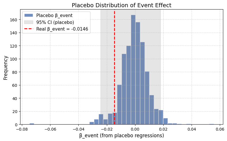
Interpretation: Placebo Test
The real β (−1.46 pp) sits comfortably inside the 95% placebo band. Similar-sized drops happen even on random, uneventful days—so we can't be sure the strike caused this particular dip.
Next we'll widen the lens to multi-day windows (e.g., ±3-day cumulative returns) to see if the market reaction was simply delayed.
Multi-day Event Window (±2 Days)
Instead of a single dummy, we add five separate indicators—two days before, the event day, and two days after—then re-estimate the model.
# Define relative days around the event
event_lags = [-2, -1, 0, 1, 2]

# Create a column for each day indicator
for lag in event_lags:
    col_name = f"event_{'m' + str(abs(lag)) if lag < 0 else lag}"
    returns[col_name] = 0
    event_idx = returns.index.get_loc(event_date)
    if 0 <= event_idx + lag < len(returns):
        lag_date = returns.index[event_idx + lag]
        returns.loc[lag_date, col_name] = 1

# Fit regression with lag dummies
cols = ['VOO', 'VXUS'] + [f"event_{'m' + str(abs(l)) if l < 0 else l}" for l in event_lags]
X = sm.add_constant(returns[cols])
y = returns['EIS']
model_lags = sm.OLS(y, X).fit()
print(model_lags.summary())

# Compute cumulative abnormal return (CAR) for +1 to +2 days
X_no_event = X.copy()
for c in X.columns:
    if c.startswith('event_'):
        X_no_event[c] = 0
returns['abnormal'] = y - model_lags.predict(X_no_event)
car = returns.iloc[event_idx+1:event_idx+3]['abnormal'].sum()
print(f"CAR (+1 to +2): {car:.4f}")
The chart below plots each lag coefficient with 95 % confidence intervals:
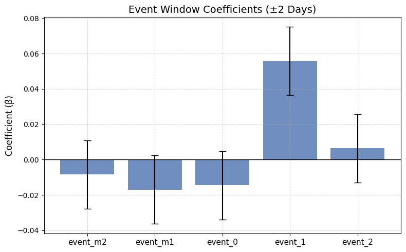
Interpretation: Event Window
• The day after the strikes (event + 1) shows a strong positive abnormal return (~ +5.6 pp) that is highly significant.
• Pre-event and event-day coefficients remain modest and insignificant.
• The cumulative abnormal return from +1 to +2 days is positive, reinforcing the idea of a quick rebound rather than a lasting sell-off.
Final Thoughts
Markets didn't crash on the strike day; if anything, they surged the day after. Placebo tests show the initial dip was indistinguishable from routine noise, and the multi-day window reveals a decisive rebound—suggesting investors quickly regained confidence.
Conclusion: Event-study techniques, paired with placebo inference, help separate signal from static when markets react to real-world shocks.